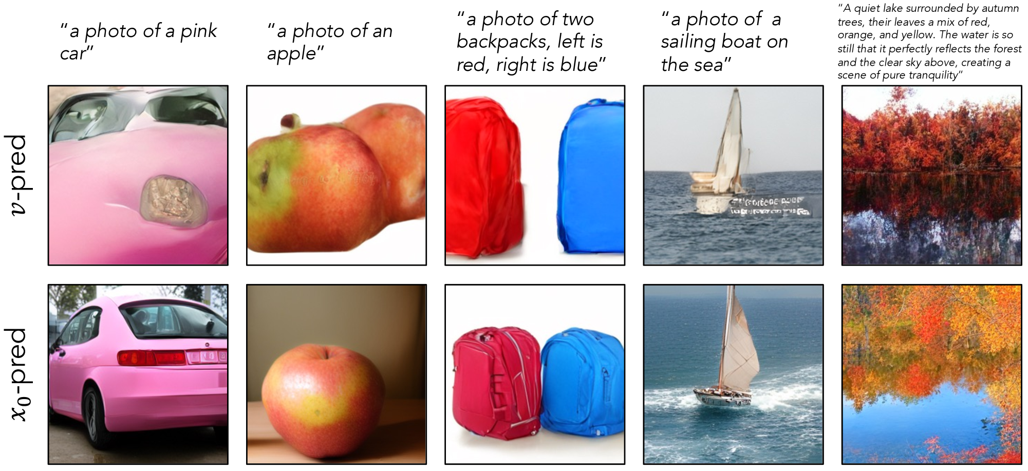
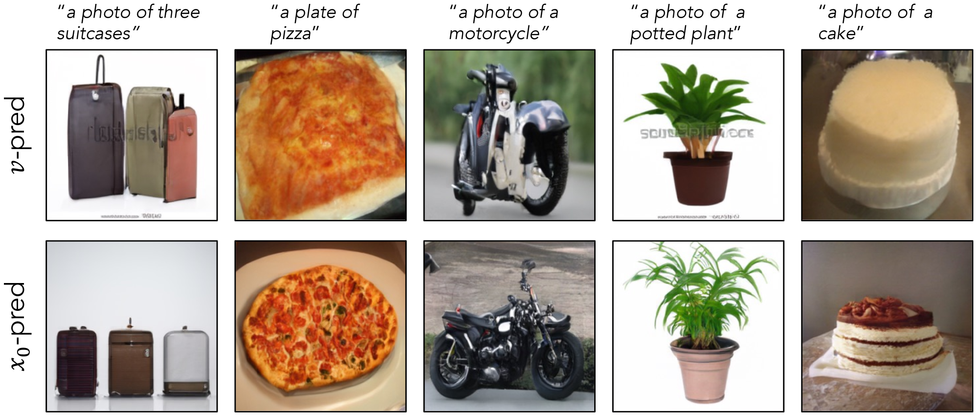
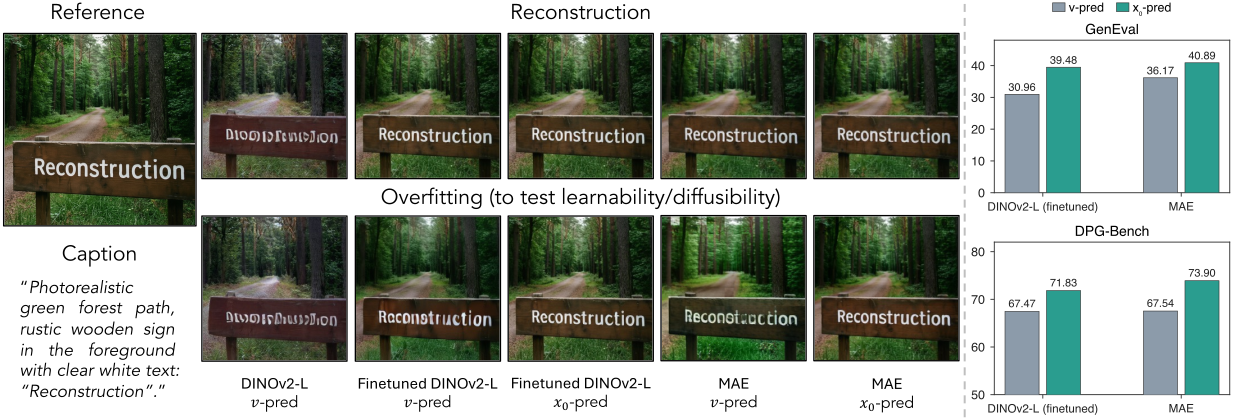
On the Diffusibility of High-Dimensional Latents

Reconstruction and learnability of high-dimensional representation autoencoders. Reconstruction-tuned tokenizers (finetuned DINOv2-L, MAE-RAE) reconstruct more faithfully than frozen DINOv2-L, yet standard flow matching \(\boldsymbol{v}\)-prediction converges slowly in their feature spaces, even in a single-image overfitting test. \(\boldsymbol{x}_0\)-prediction mitigates this optimization difficulty (left). The advantage carries over to text-to-image generation on GenEval and DPG-Bench (right).

Abstract

Representation Autoencoders (RAEs) enable diffusion models to operate in the feature spaces of pretrained visual encoders. However, many off-the-shelf encoders are not optimized for faithful reconstruction and often discard fine-grained visual details. Finetuning these encoders for image reconstruction can recover such details, but we show that it also reduces the effective dimensionality of the resulting representation space. We analyze how this altered geometry affects generation in high-dimensional feature spaces. Under this geometry, standard velocity prediction in flow matching can require the model to fit orthogonal noise directions outside the low-dimensional signal manifold, making optimization inefficient. This motivates the clean data parameterization (\(\boldsymbol{x}_{0}\)-prediction), which focuses learning on the underlying signal manifold. Across experiments with multiple reconstruction-finetuned feature sets, we show that \(\boldsymbol{x}_{0}\)-prediction consistently improves text-to-image generation performance.

Method

We study text-to-image generation directly in high-dimensional, reconstruction-tuned representation spaces. Click through the tabs below to learn more about each part: our empirical analysis of why these spaces are hard to diffuse in (1), the mathematical picture behind this difficulty and its fix (2), and the resulting text-to-image framework (3).

Reconstruction tuning collapses effective dimensionality

Finetuning an encoder with a reconstruction objective recovers the high-frequency details that semantic latents miss — but as the teaser shows, standard flow matching \(\boldsymbol{v}\)-prediction becomes surprisingly hard to optimize in the finetuned space. To understand why, we analyze the singular value spectrum of patch embeddings across encoders.

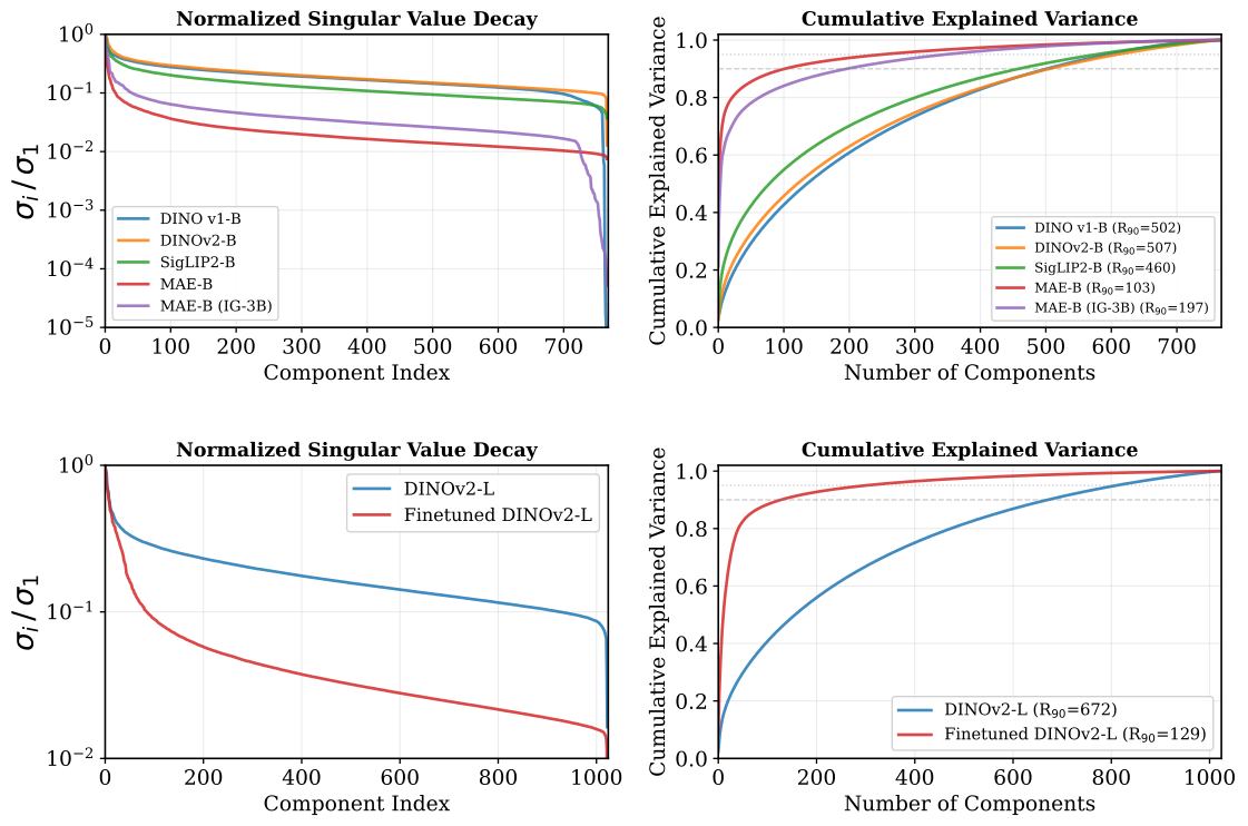
What is effective dimensionality? We extract L2-normalized per-patch features for 200k ImageNet patches, stack them into \(H \in \mathbb{R}^{N \times D}\), and compute singular values \(\sigma_{1} \geq \dots \geq \sigma_{D}\) via SVD. With total energy \(E = {\textstyle\sum}_{i=1}^{D}\sigma_{i}^{2}\), the cumulative energy of the top \(k\) components and the effective dimensionality are \[ C(k) = \frac{\sum_{i=1}^{k}\sigma_{i}^{2}}{E}, \qquad R_{\tau} = \min \{ k \mid C(k) \geq \tau \}, \] i.e., \(R_{\tau}\) is the minimum number of components explaining at least \(\tau\%\) of the variance. We evaluate \(\tau \in \{90, 95, 99\}\).

Effective dimensionality and reconstruction (PSNR) on the ImageNet validation set. Top group: frozen encoders with decoders from RAE (* our own decoder for MAE-B from MAWS, same architecture). Bottom group: DINOv2-L with a frozen vs. finetuned encoder.

Tokenizer/Encoder	Training dataset	Dimensions				Reconstruction (PSNR)
Tokenizer/Encoder	Training dataset	Full	\(R_{90}\)	\(R_{95}\)	\(R_{99}\)	Reconstruction (PSNR)
DINOv1-B	IN-1k	768	502	595	701	—
DINOv2-B-RAE	LVD-142M	768	507	611	726	18.85
SigLIP2-B-RAE	WebLI	768	460	578	715	19.10
MAE-B-RAE	IN-1k	768	103	252	578	28.13
MAE-B-IG-3B*	Instagram-3B	768	197	348	595	27.67
DINOv2-L	LVD-142M	1024	672	811	965	17.34
Finetuned DINOv2-L	—	1024	129	302	726	29.12

Semantically pretrained encoders (DINOv1, DINOv2, SigLIP2) keep effective dimensionality high relative to the full feature dimension — DINOv1 does so despite being pretrained only on ImageNet. Encoders trained for reconstruction do not: MAE exhibits much lower effective dimensionality even when pretrained on Instagram-3B, and finetuning DINOv2-L for reconstruction drops \(R_{90}\) from 672 to 129. When an encoder is trained for reconstruction, the ratio of effective dimensionality to the full feature dimension shrinks significantly.

Normalized singular value decay and cumulative explained variance

The normalized singular values of MAE decay rapidly, a bottleneck that persists even with Instagram-3B pretraining, and finetuned DINOv2-L needs far fewer principal components than the frozen model to capture the same variance. A potential reason: to reconstruct, the encoder must capture significant high-frequency information — and since natural images reside near a low-dimensional manifold, the features are forced to mimic this lower-dimensional distribution.

Velocity prediction wastes capacity on orthogonal noise

Setup. Flow matching constructs the noisy input by linear interpolation between clean data \(\boldsymbol{x}_{0} \sim p_{\text{data}}(\boldsymbol{x})\) and isotropic Gaussian noise \(\boldsymbol{\epsilon} \sim \mathcal{N}(0, \mathbf{I})\): \(\boldsymbol{z}_{t} = (1-t)\boldsymbol{x}_{0} + t\boldsymbol{\epsilon}\), and standard practice trains the model to predict the velocity \(\boldsymbol{v} = \boldsymbol{\epsilon} - \boldsymbol{x}_{0}\). Alternatively, the model can output the clean data \(\boldsymbol{x}_{\theta}\) directly (\(\boldsymbol{x}_{0}\)-prediction) while still being trained with the velocity loss via the transformation \(\boldsymbol{v}_{\theta} = (\boldsymbol{z}_{t}-\boldsymbol{x}_{\theta})/t\): \[ \mathcal{L} = \mathbb{E}_{t, \boldsymbol{x}_{0}, \boldsymbol{\epsilon}} \left\| \boldsymbol{v}_\theta(\boldsymbol{z}_{t}, t) - \boldsymbol{v} \right\|^2 = \mathbb{E}_{t, \boldsymbol{x}_{0}, \boldsymbol{\epsilon}} \left\| \frac{\boldsymbol{x}_{0} - \boldsymbol{x}_{\theta}}{t}\right\|^2. \]

A low-dimensional subspace model. Our analysis suggests that high-dimensional encoders trained or finetuned for an image reconstruction objective concentrate near a low-dimensional subspace. Assume the observed high-dimensional feature \(\boldsymbol{x}_{0} \in \mathbb{R}^{h}\), extracted by a visual encoder, is generated from a true latent variable \(\boldsymbol{c}_{0} \in \mathbb{R}^{l}\) via the linear mapping \(\boldsymbol{x}_{0} = Q\boldsymbol{c}_{0}\), where the columns of \(Q \in \mathbb{R}^{h \times l}\) form an orthonormal basis for the subspace (i.e., \(Q^{\top} Q = I_{l}\)). The noisy input \(\boldsymbol{z}_{t}^{h} = (1-t)\boldsymbol{x}_{0} + t\boldsymbol{\epsilon}_{h}\) then decomposes into a manifold component and a normal component: \[ \boldsymbol{z}_{t}^{h} = Q\underbrace{\big((1-t)\boldsymbol{c}_{0} + t\boldsymbol{\epsilon}_{l}\big)}_{\boldsymbol{z}_{t}^{l}\ \text{(manifold)}} + \; t\underbrace{\boldsymbol{\epsilon}_{\perp}}_{\text{(normal)}}, \qquad \boldsymbol{\epsilon}_{\perp} = (I - QQ^{\top})\boldsymbol{\epsilon}_{h}, \] and we have \((I-QQ^{\top})\boldsymbol{z}_{t}^{h} = t\boldsymbol{\epsilon}_{\perp}\).

Velocity prediction in high dimensions. The model that predicts velocity in the high-dimensional space is defined as \(\boldsymbol{v}_{\theta}^{h}(\boldsymbol{z}_{t}^{h}, t) = \mathbb{E}[\boldsymbol{\epsilon}_{h} - \boldsymbol{x}_{0} \mid \boldsymbol{z}_{t}^{h}] = \mathbb{E} [ Q (\boldsymbol{\epsilon}_{l} - \boldsymbol{c}_{0}) + \boldsymbol{\epsilon}_{\perp} \mid \boldsymbol{z}_{t}^{h}]\). Therefore, we can obtain \[ \begin{aligned} \boldsymbol{v}_{\theta}^{h}(\boldsymbol{z}_t^{h}, t) &= \mathbb{E} [ Q (\boldsymbol{\epsilon}_{l} - \boldsymbol{c}_{0}) \mid \boldsymbol{z}_{t}^{h}] + \mathbb{E} [ \boldsymbol{\epsilon}_{\perp} \mid \boldsymbol{z}_{t}^{h}] \\ &= Q\boldsymbol{v}_{\theta}^{l}(Q^\top \boldsymbol{z}_t^{h}, t) + \frac{1}{t}(I - QQ^\top)\boldsymbol{z}_{t}^{h}. \end{aligned} \] The second term comes from \(\boldsymbol{\epsilon}_{\perp}\), which is introduced by \(\boldsymbol{\epsilon}_{h}\) in the vanilla velocity prediction training target and is largely uninformative about the clean representation. When the feature dimension is much higher than the intrinsic dimension (\(h \gg l\)), the model needs to allocate substantial capacity to fitting \(\frac{1}{t}(I - QQ^\top)\boldsymbol{z}_{t}^{h}\), making optimization inefficient and degrading sample quality.

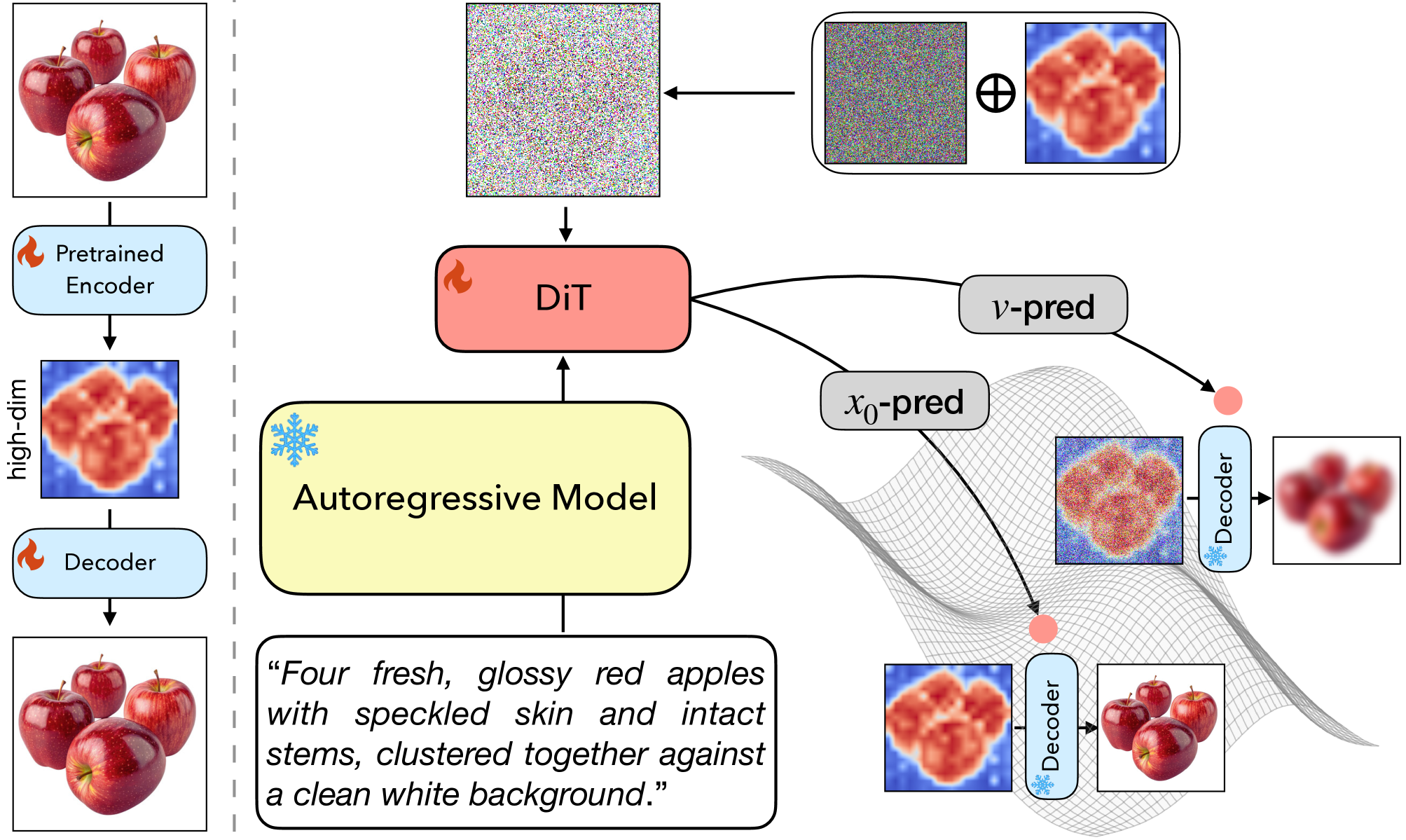
\(\boldsymbol{x}_{0}\)-prediction bypasses the orthogonal noise. To avoid this, we employ the model to predict \(\boldsymbol{x}_{0}\) directly: \[ \boldsymbol{x}_{\theta}^{h}(\boldsymbol{z}_{t}^{h}, t) = \mathbb{E}[\boldsymbol{x}_{0} \mid \boldsymbol{z}_{t}^{h}] = \mathbb{E}[Q\boldsymbol{c}_{0} \mid Q\boldsymbol{z}_{t}^{l} + t\boldsymbol{\epsilon}_{\perp}] = \mathbb{E}[Q\boldsymbol{c}_{0} \mid Q\boldsymbol{z}_{t}^{l},\; t\boldsymbol{\epsilon}_{\perp}]. \] Since \(Q\boldsymbol{c}_{0}\) is independent of \(t\boldsymbol{\epsilon}_{\perp}\), this simplifies to \[ \boldsymbol{x}_{\theta}^{h}(\boldsymbol{z}_{t}^{h}, t) = \mathbb{E}[Q\boldsymbol{c}_{0} \mid Q\boldsymbol{z}_{t}^{l}] = Q\,\mathbb{E}[\boldsymbol{c}_{0} \mid Q\boldsymbol{z}_{t}^{l}] = Q\,\boldsymbol{x}_{\theta}^{l}(\boldsymbol{z}_{t}^{l}, t). \] Directly modeling \(\boldsymbol{x}_{0} \in \mathbb{R}^{h}\) in the high-dimensional space can thus predict \(\boldsymbol{c}_{0} \in \mathbb{R}^{l}\) more efficiently — the orthogonal noise directions never need to be modeled explicitly — especially when \(h \gg l\).

Text-to-image generation with strong-reconstruction representation autoencoders

Method overview. (a) Tokenizer: we unfreeze the pretrained visual encoder when training the decoder for reconstruction, then use the high-dimensional representation from the finetuned encoder as the latent. (b) Text-to-image generation framework: we use an autoregressive model and query tokens to extract text embeddings as conditioning for the DiT. Due to the low-dimensional manifold property, we employ \(\boldsymbol{x}_{0}\)-prediction to train the text-to-image DiT more efficiently.

Strong-reconstruction tokenizer. To obtain a representation autoencoder with strong reconstruction, we unfreeze the encoder (e.g., DINOv2-L) during reconstruction training. Besides the reconstruction loss, we also leverage a semantic preservation loss to prevent collapse. Specifically, for each image \(I\), the feature extracted by the original frozen encoder \(g\) supervises the finetuned encoder \(g'\): \[ \mathcal{L}_{\text{FT}} = \|g(I) - g'(I)\|^2 + \mathcal{L}_{\text{recon}}, \] where \(\mathcal{L}_{\text{recon}}\) consists of pixel-level \(L_{1}\), perceptual, and adversarial losses.

Text-to-image generation architecture. The high-dimensional visual features produced by the strong-reconstruction representation autoencoder are used as latents for diffusion. For the generation framework, we use a frozen pretrained vision-language model (VLM) as the autoregressive model. Learnable query tokens are employed to extract text information as conditioning for a randomly initialized diffusion transformer (DiT).

\(\boldsymbol{x}_{0}\)-prediction for representation latents. Given a text-image pair \((\boldsymbol{I}_{i}, \boldsymbol{T}_{i})\), extracted text embeddings act as the condition \(\boldsymbol{y}_{i}\) for the diffusion transformer \(\boldsymbol{x}_{\theta}\), and the feature \(\boldsymbol{h}_{i} = g(\boldsymbol{I}_{i})\) produced by the representation autoencoder \(g\) is used as the latent for diffusion. Given the noisy input \(\boldsymbol{h}_{i,t} = (1-t)\boldsymbol{h}_{i,0} + t\boldsymbol{\epsilon}\), the DiT is trained to denoise noisy image representations: \[ \mathcal{L}_{\text{Diff}} = \mathbb{E}_{t, \boldsymbol{h}_{i,0}, \boldsymbol{\epsilon}} \left\| \frac{\boldsymbol{h}_{i, 0} - \boldsymbol{x}_{\theta}(\boldsymbol{h}_{i,t}, t, \boldsymbol{y}_{i})}{t}\right\|^2, \] where \(\boldsymbol{h}_{i,0} := \boldsymbol{h}_{i}\) is the clean feature. In practice, we clamp \(t\) to a minimum of 0.05 to prevent numerical instability.

Experiments

We use a frozen Qwen3-VL-2B-Instruct as the autoregressive model and a 1B-parameter Lumina-Next DiT trained from scratch on a 34M subset of the public BLIP3-o pretraining dataset at 256×256 resolution. We report GenEval and DPG-Bench for text-image alignment, and COCO-30k FID for image quality. Click through the tabs below to see each comparison.

\(\boldsymbol{x}_{0}\)-prediction beats \(\boldsymbol{v}\)-prediction for finetuned DINOv2-L

Finetuning DINOv2-L by reconstruction and performing standard \(\boldsymbol{v}\)-prediction deteriorates performance on all three benchmarks — the diffusibility of the representation space decreases. Switching to \(\boldsymbol{x}_{0}\)-prediction boosts performance by a large margin and surpasses the original DINOv2-L. The low-dimensional variant (gray) achieves stronger text alignment, but this compression costs image quality: our unbottlenecked \(\boldsymbol{x}_{0}\) variant achieves better FID (16.80 vs. 17.64).

Tokenizer	Dimension	Pred. type	GenEval↑	DPG-Bench↑	COCO-30k FID↓
FT-DINOv2-L-low-dim	32	\(\boldsymbol{v}\)	40.99	73.04	17.64
DINOv2-L	1024	\(\boldsymbol{v}\)	37.63	70.21	18.34
FT-DINOv2-L	1024	\(\boldsymbol{v}\)	30.96	67.47	29.97
FT-DINOv2-L	1024	\(\boldsymbol{x}_{0}\)	39.48	71.83	16.80

Qualitative comparison of x0 and v predictions for finetuned DINOv2-L

\(\boldsymbol{x}_{0}\)-prediction maintains strong structural integrity (e.g., "a photo of a pink car"), while \(\boldsymbol{v}\)-prediction produces amorphous, blob-like structures.

\(\boldsymbol{x}_{0}\)-prediction also wins for MAE-RAE

The MAE encoder is pretrained with a reconstruction objective and has low effective dimensionality, as shown in our analysis. As predicted, \(\boldsymbol{x}_{0}\)-prediction improves text-to-image generation on all three benchmarks, with better object structure and richer details in the samples.

Tokenizer	Dimension	Pred. type	GenEval↑	DPG-Bench↑	COCO-30k FID↓
MAE-B-RAE	768	\(\boldsymbol{v}\)	36.17	67.54	22.20
MAE-B-RAE	768	\(\boldsymbol{x}_{0}\)	40.89	73.90	17.24

Qualitative comparison of x0 and v predictions for MAE

Generated examples comparing \(\boldsymbol{x}_{0}\) and \(\boldsymbol{v}\) prediction targets with the MAE-RAE tokenizer.

Reconstruction still matters for generation

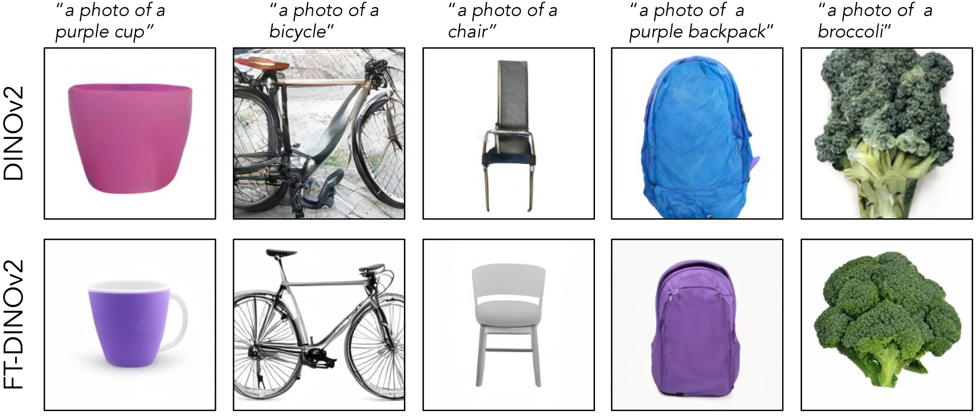
Comparing the original DINOv2-L (\(\boldsymbol{v}\)-prediction) against our finetuned DINOv2-L (\(\boldsymbol{x}_{0}\)-prediction): the finetuned tokenizer wins on all three benchmarks (see tab 1), indicating that tuning the encoder by reconstruction helps generation. The original DINOv2-L fails to capture correct color information (e.g., "a photo of a purple backpack") or object integrity when the texture is complicated (e.g., "a photo of a bicycle").

Qualitative comparison of DINOv2-L and finetuned DINOv2-L

The finetuned encoder leads to better structural integrity and color alignment.

Scaling to a Larger Dataset

We further train a diffusion model with \(\boldsymbol{x}_{0}\)-prediction using the finetuned DINOv2 tokenizer on a larger internal 90M dataset, while keeping the remaining hyperparameters unchanged. Following Scale-RAE, we then finetune the pretrained model on BLIP3o-60k at 256 resolution, and additionally finetune a high-resolution variant at 512 resolution. We include Scale-RAE as a reference. These results suggest that our method has potential scalability and could achieve competitive performance for text-to-image generation.

Scaling to a larger dataset. We train our method on a larger-scale dataset and perform supervised finetuning (SFT) at resolutions of 256 and 512. The asterisk (*) denotes our own SFT implementation. Best are highlighted in bold.

Method	DiT size	Training dataset	Latent dim.	Res.	GenEval↑	DPG-Bench↑
Ours	1B	90M	1024	256	43.84	76.15
Ours	1B	90M + SFT 60k	1024	256	78.62	80.13
Ours (512)	1B	90M (256) + SFT 60k (512)	1024	512	79.69	81.15
Scale-RAE*	2.4B	64M + SFT 60k	1152	224	77.43	78.47

Acknowledgements

We thank Sicheng Mo, Xichen Pan, Eli Shechtman, Krishna Kumar Singh, and Nicolas Dufour for their valuable discussions and help. This work was supported in part by NSF CAREER #2339071.

BibTeX

@article{feng2026on,
  title={On the Diffusibility of High-Dimensional Latents},
  author={Feng, Chao and Xu, Zhiyang and Chen, Bowei and Xiong, Yuanjun and Wang, Xiyao and Wang, Jui-Hsien and Zhang, Richard and Lin, Zhe and Owens, Andrew and Li, Yijun},
  journal={European Conference on Computer Vision (ECCV)},
  year={2026},
}